Chapter 3 Linear Regression

What is linear regression?

“a very simple approach for supervised learning”
“a useful tool for predicting a quantitative response”
widely used statistical learning method
a special case of more generalized learning methods
Useful for answering many different types of questions

Advantages

Simplicity
- Conceptual: based on averages (or “expectations” in econometrics)
- Procedural: there are closed form solutions for estimating parameters
Interpretable
- There are meaningful visualizations and interpretations of model results
- It is possible to address many types of questions, and apply statistical tests to judge results including:
  1. Is there a relationship between predictors and response variables?
  2. How strong is the relationship?
  3. Which predictors are related to the response?
  4. How accurate are the estimated model parameters?
  5. How accurate are the predictions generated by the model?
  6. Is the model a good fit?
  7. Are there interactions among the predictors?

3.1 Simple linear regression

Simple linear regression predicts a quantitative response \(y\) on the basis of a single predictor, \(x\), assuming that there is a linear relationship between \(y\) and \(x\) in the form:

\[ \begin{array}{rcl} y &=& \beta_0 + \beta_{1}x + \epsilon \\ &\textrm{or}& \\ y &\approx& \beta_0 + \beta_{1}x \end{array} \]

Read as: “regressing \(y\) on \(x\)”, “regressing \(y\) onto \(x\)”, or “\(y\) is approximately modeled as a linear function of \(x\)”

This equation describes the population regression line: the best linear approximation of the true relationship between \(y\) and \(x\). The model parameters (or coefficients), \(\beta_0\) and \(\beta_1\), are unknown constants and the error term, \(\epsilon\), is not measurable in practice.

\(y\): the observed true value of \(y\)
\(\beta_0\): the intercept, or the expected value of \(y\), when \(x\) is 0
\(\beta_1\): the slope, or the expected change in \(y\) per unit change in \(x\), or \(\frac{\Delta y}{\Delta x}\)
\(\epsilon\): irreducible error, or variation in \(y\) that can not be accounted for by the model

3.1.1 Estimating Coefficients

In practice \(\beta_0\) and \(\beta_1\) are unknown constants that must be estimated based on available data using some procedure.

Each \((x_i, y_i)\) pair represents an example observation drawn from the population of possibilities for the joint distribution of \(X\) and \(Y\).
Based on many (\(n\)) examples, develop estimates for \(\hat{\beta}_0\) and \(\hat{\beta}_1\).
Then compute \(\hat{y}_i\), which is the value for \(y_i\) predicted by the model based on \(x_i\) (where \(i \in \{1 \ldots n\}\)).

\[ \hat{y}_i \approx \hat{\beta}_0 + \hat{\beta}_1 x_i \]

The prediction is an approximation is unlikely to be exactly equal to the actual value. The difference is called the residual. For a particular example observation, \(i\), the residual is computed as:

\[ e_i = y_i - \hat{y}_i \]

Better estimates of the parameters \(\beta_0\) and \(\beta_1\) will yield better predictions for \(y\) and, therefore, smaller residuals. The residual sum pf squares (RSS) is a measure of the overall magnitude of the prediction error for a particular set of coefficients and training data. The lower the RSS, the better the estimates should be (assuming the model is correctly specified, etc.).

\[ \begin{array}{rcl} RSS &=& \sum_{i}^{n} e_{i}^{2} \\ &=& \sum_{i}^{n} (y_i -\hat{y}_i)^2 \\ &=& \sum_{i}^{n} (y_i - \hat{\beta}_0 + \hat{\beta}_1 x_i)^2 \end{array} \]

Minimizing the RSS is accomplished by choosing appropriate values for \(\hat{\beta}_0\) and \(\hat{\beta}_1\), which are estimates for the true (but unknown) population parameters, \(\beta_0\) and \(\beta_1\). This method is referred to as the least squares approach in the text.

3.1.2 Simulated Data Example

set.seed(20210707)

model: \(y = \beta_0 + \beta_1 x + \epsilon\)
parameters: \(\beta_0\) = 2 and \(\beta_1\) = 3.

Simulate drawing a sample from the population by generating data

# Number of observations
n <- 100

# random variable x
x <- runif(n)

# True slope and intercept of line
beta <- c(2, 3)

# irreducible error
epsilon <- rnorm(n)

# True value of y
y <- beta[1] + beta[2] * x + epsilon

First few rows of the simulated data sample

tibble(y, x, epsilon) %>%
    head() %>%
    kable(booktabs = TRUE)

y	x	epsilon
4.299174	0.8543299	-0.2638157
1.188886	0.1168752	-1.1617401
5.271001	0.6867674	1.2106981
3.357570	0.0163384	1.3085549
2.984540	0.3480136	-0.0595011
4.802275	0.6009924	0.9992976

Minimize RSS to compute least squares estimates for \(\hat{\beta_0}\) and \(\hat{\beta_1}\)

# residual sum of squares formula
rss <- function(...) {
    beta <- c(...)
    sum((y - (beta[1] + beta[2] * x))^2)
}

Try guessing the parameters that will minimize RSS for the sample

rss(0, 1)
rss(1, 2)
rss(2, 3)
rss(1.8, 3.3)

tibble(beta_0 = c(0, 1, 2, 1.8), beta_1 = c(1, 2, 3, 3.3)) %>%
    group_by(beta_0, beta_1) %>%
    mutate(RSS = rss(beta_0, beta_1)) %>%
    ungroup() %>%
    kable()

beta_0	beta_1	RSS
0.0	1.0	1094.7367
1.0	2.0	363.2831
2.0	3.0	102.3890
1.8	3.3	101.1695

Surprisingly (perhaps) using \(\hat{\beta_0}\) = 2 and \(\hat{\beta_1}\) = 3 does not yield the lowest RSS for the sample data even though these are the exact parameters \(\beta_0\) and \(\beta_1\) used to generate the sample observations. This is because irreducible error component is not observed and our sample size is limited.

Instead of guessing we can use R to automatically choose beta to minimize RSS. The optim() can do this.

fit <- optim(par = c(0, 1), fn = rss)
fit$par

## [1] 1.778687 3.545284

3.1.3 Closed-form solution

Applying some algebra and calculus to the RSS formula yields the following exact solutions for estimating \(\hat{\beta_0}\) and \(\hat{\beta_1}\) that will minimize RSS

\[ \begin{array}{rcl} \hat{\beta_1} & = & \frac{\sum_{i=1}^{n} (x_i - \bar{x})(y_i - \bar(y)) }{ \sum_{i=1}^{n} (x_i - \bar{x})^2 } \\ \hat{\beta_0} & = & \bar{y} - \hat{\beta_1}\bar{x} \\ \end{array} \]

b1 <- sum((x - mean(x)) * (y - mean(y))) / sum((x - mean(x))^2)
b1

## [1] 3.544119

b0 <- mean(y) - (b1 * mean(x))
b0

## [1] 1.779281

Estimated model using least squares method:

\(\hat{y}\) = 1.78 + 3.54 \(x\)

We can also use the lm() function to estimate the parameters

lm(y ~ x)

## 
## Call:
## lm(formula = y ~ x)
## 
## Coefficients:
## (Intercept)            x  
##       1.779        3.544

3.2 Assessing Accuracy of Coefficients

The goal is to estimate pthe arameters of the actual population regression function based on a sample

Since we have estimated our parameters based on a sample, there is likely to be some error.

simulate_data <- function(beta = c(0, 0), n = 100, sd = 1) {
    # column dimension
    m <- length(beta)
    
    # Population parameters
    beta <- matrix(beta, nrow = 1, dimnames = list(NULL, paste0("beta_", seq_along(beta)-1)))
    
    # Sample Data
    X <- matrix(
        data = c(rep(1, n),                    # Assign a constant term for x_0 
                 rnorm((m-1) * n, sd = sd)),   # random normals for remaining x
        ncol = m, nrow = n,
        byrow = FALSE,
        dimnames = list(NULL, paste0("x_", seq_along(beta)-1))
    )

    # Irreducible error 
    e <- matrix(rnorm(n, sd = sd), ncol = 1, dimnames = list(NULL, "e"))
    
    # Compute y
    y <- X %*% t(beta) + e
    colnames(y) <- "y"

    # Return a data frame, drop the constant
    data.frame(cbind(y, X, e))[, -2]
}

#test <- simulate_data(beta = c(2, 3), n = 1000)
#test

Here is a plot of linear function with the parameters we estimated, compared with the population regression function.

# Replicate Figure 3.3

# Generate 1 sample and plot
simulate_data(beta = c(2, 3), n = 100, sd = 3) %>%
ggplot(mapping = aes(x = x_1, y = y)) +
    geom_abline(slope = 3, intercept = 2, color = "red") +
    geom_point() +
    geom_smooth(method = "lm", se = FALSE, size = 0.5) +
    scale_x_continuous(limits = c(-2, 2)) +
    scale_y_continuous(limits = c(-10, 10)) +
    labs(title = "Population Regression Line and Estimated Regression Line")

## `geom_smooth()` using formula 'y ~ x'

## Warning: Removed 44 rows containing non-finite values (stat_smooth).

## Warning: Removed 44 rows containing missing values (geom_point).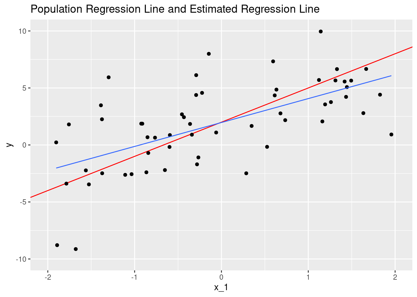

Resampling several times, we find that we end up with several estimated functions (sets of parameters)

# Generate 10 samples and plot
map_df(1:10, ~ simulate_data(beta = c(2, 3), n = 100, sd = 3), .id = "sample") %>%
    mutate(sample = as.factor(as.numeric(sample))) %>%
ggplot(mapping = aes(x = x_1, y = y, color = sample)) +
    geom_abline(slope = 3, intercept = 2, color = "red") +
    geom_smooth(method = "lm", se = FALSE, size = 0.5) +
    scale_x_continuous(limits = c(-2, 2)) +
    scale_y_continuous(limits = c(-10, 10)) +
    labs(title = "Regression lines for 10 simulated datasets")

## `geom_smooth()` using formula 'y ~ x'

## Warning: Removed 549 rows containing non-finite values (stat_smooth).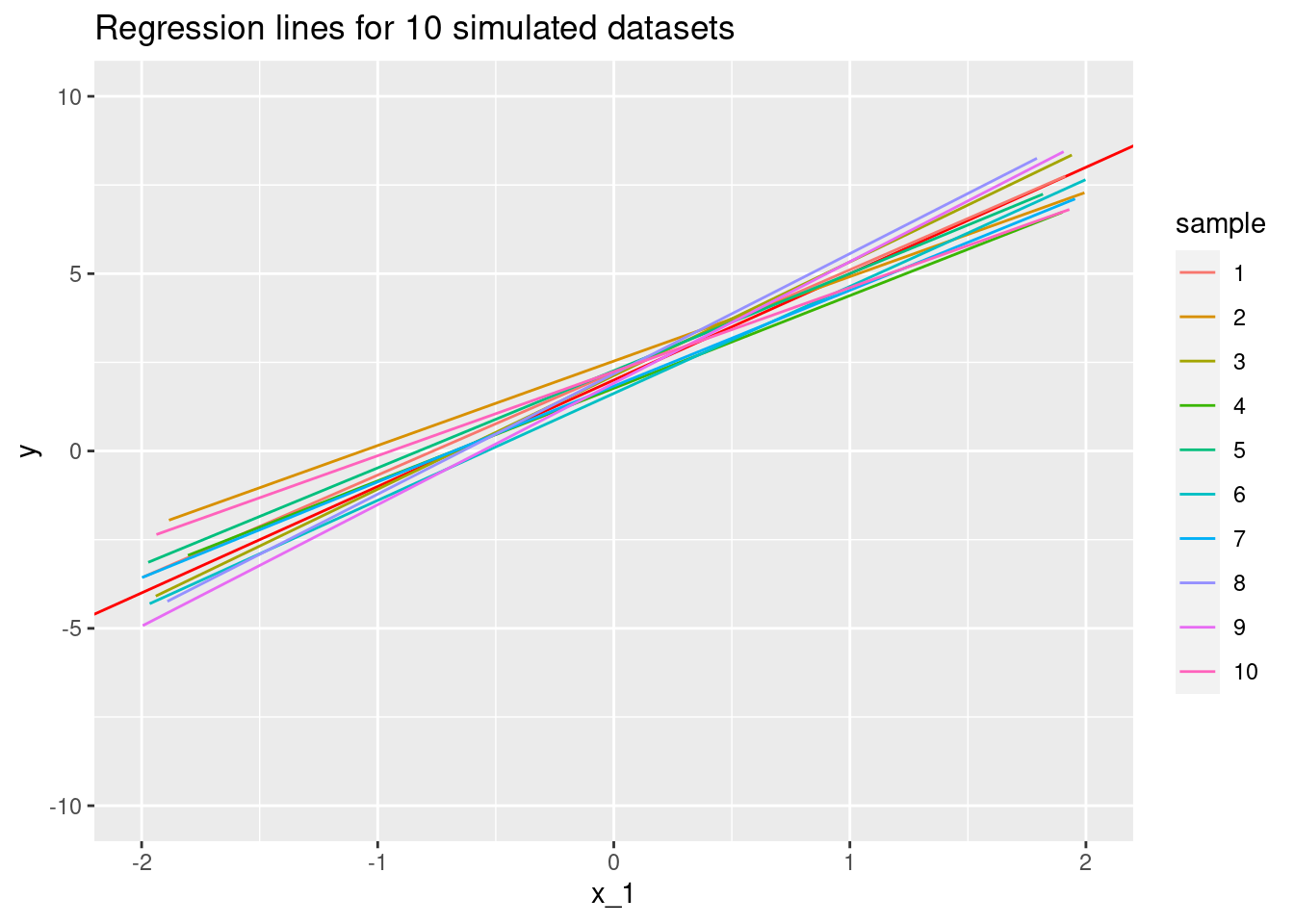

How can we assess accuracy? Statisics!

pmap_dfr(
    expand.grid(n = c(10, 50, 100), k = c(10, 50, 100), N = 10000, mean = 0), 
    generate_sample_means
) %>% 
    law_of_large_n_gridplot_dots()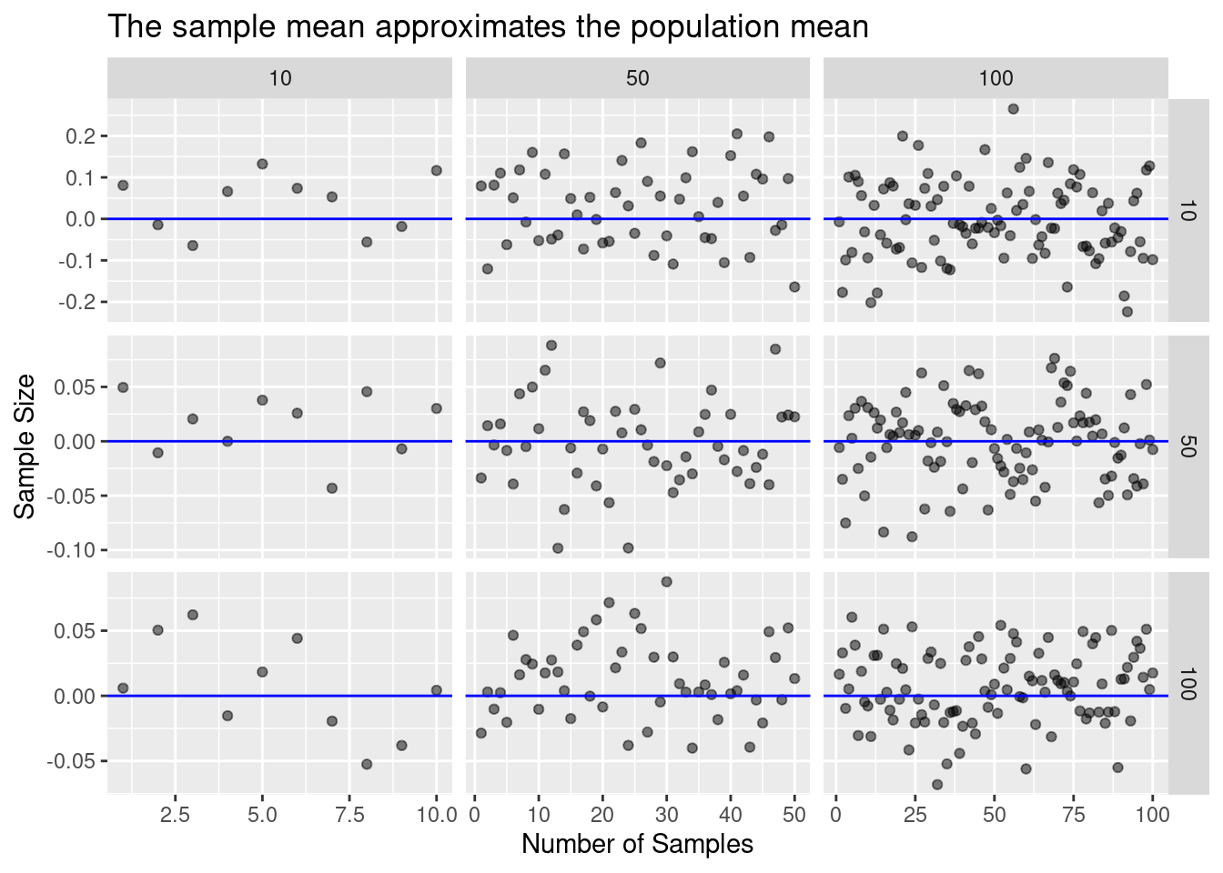

pmap_dfr(
    expand.grid(n = c(10, 50, 100), k = c(10, 50, 100), N = 10000, mean = 0), 
    generate_sample_means
) %>% 
    law_of_large_n_gridplot_density()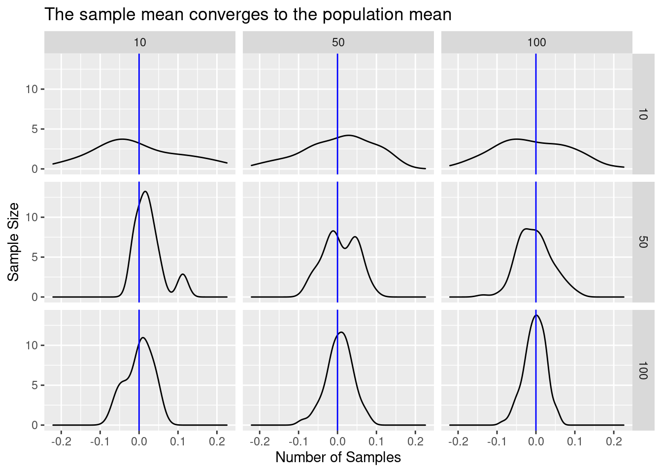

pmap_dfr(
    expand.grid(n = c(10, 50, 100), k = c(10, 50, 100), N = 10000, mean = 0), 
    generate_sample_means
) %>% 
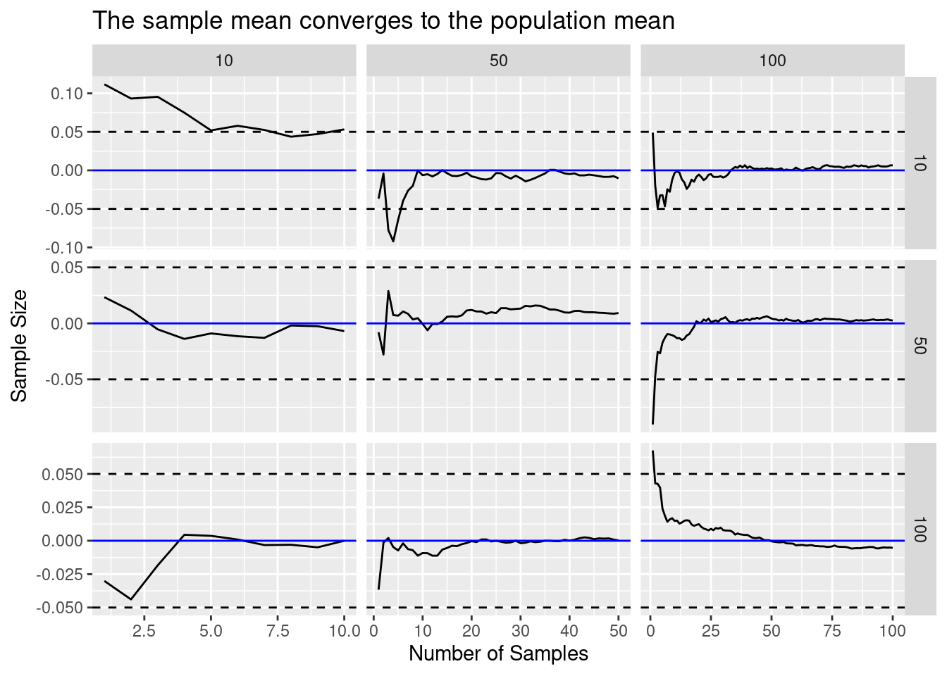
    law_of_large_n_gridplot()

ISLR Notes